Adaptive Sampling for DER Baseline Estimation: A Fair and Scalable Sampling Framework

Executive Summary

This report presents an innovative statistical sampling framework for Distributed Energy Resource (DER) baselining that addresses the industry's critical needs for accuracy and scalability. Our dynamic sampling methodology enables grid operators to establish reliable baselines across diverse DER types and aggregation sizes.

Key innovations include a probability-based sampling approach that continuously cycles DERs between baseline and treatment groups and a compensation framework that prevents manipulation. The sampling framework scales effectively using relative metrics rather than absolute values, while the compensation strategy incentivizes truthful forecasts by penalizing baseline errors. Together, these mechanisms ensure system integrity while enabling seamless integration of new DERs and varying aggregation sizes without compromising baseline accuracy.

Introduction

Definitions and Terminology

• We define distributed energy resources (DER) as any controllable generation, energy consumption device, or energy storage device, such as curtailable solar, batteries, EVs, water heaters, HVAC systems, pool pumps, heat pumps, etc.
• We refer to a DER event as the act of controlling distributed energy resources (DER) to reach a desired result, such as load shedding, load build, and fast frequency response. We use the terms event, treatment, and intervention interchangeably.
• We define DER baselining as establishing the counterfactual for a DER event, that is, determining how much energy a DER would have consumed/generated if no event had occurred.
• Normal operating conditions (NOC) refer to the energy consumption/generation of the DER when not influenced by a DER event. The DER baseline estimates the energy consumption/generation under NOC.
• The event impact is the difference between the observed consumption/generation of the DERs during the event compared to their baselines.
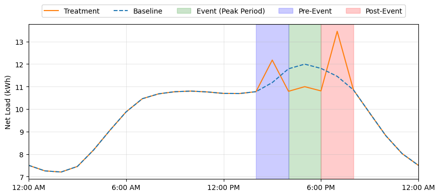
• DER behavior can be affected before, after, and during an event. We refer to this change in behavior as event-induced bias.
• The treatment group contains the DERs that participate in a DER event.
• The baseline group contains the DERs that do not participate in a DER event.
• A DER aggregator operates like a virtual power plant (VPP) and is in charge of controlling a group of DERs. DER aggregators typically contract with a utility and pass on their profits to the owners of the DERs they control. In this report, we assume all DERs are under the control of an aggregator.

Motivation

Accurate DER baselining is essential for grid operators managing diverse energy resources across large geographic regions. As utilities integrate heterogeneous combinations of demand response programs, rooftop solar installations, and electric vehicle chargers, they require reliable methods to verify real-time performance and prevent artificial manipulation of load data. Precise baseline measurements enable grid operators to distinguish genuine DER contributions from claimed performance, ensuring fair compensation while maintaining grid reliability.

The challenge is particularly complex given varying aggregation sizes, from small 0.1 MW groupings to large collections of distributed loads, each affected by changing dynamics, including seasonal factors. A robust baselining methodology must therefore adapt to these diverse conditions while providing scalable, technology-neutral solutions that can evolve with changing grid conditions and DER types.

Challenges

DER baselining is complicated by event-induced bias. DER behavior can be affected before and after an event; e.g., water heaters that are controlled to reduce load during an event may preheat to have sufficient hot water during the event; furthermore, if the water heater is deprived of sufficient hot water during the event, then it may immediately consume energy after the event (sometimes known as snapback). To estimate the baseline accurately, we would need to exclude this data from the calculation. To make things more complicated, different device types return to NOC at different rates; e.g., batteries can return to NOC almost immediately, while water heaters take longer to return to NOC. In our experience, the time it takes most device types to return to NOC is, at most, one day. Therefore, we can avoid the problem of biasing the baseline estimation with event-influenced data by having DERs wait at least one day between consecutive DER events. In this report, we discuss how we can enforce this constraint and avoid event-induced bias.

Figure 1: Event-induced bias refers to the change in DER behavior before, during, and after the event. Here, we show an example of a load shed event called from 4:00 PM to 6:00 PM. Notice that the net load during the event decreases (as expected); however, the net load before and after the event also increases

We also address the limitations of using a single fixed set of DERs to estimate the baseline. For concreteness, assume that a group of DERs is split into two groups, the treatment group, which contains the DERs that participate in an event, and the baseline group, which is assumed to be operating under NOC. The main problems with this approach are:

• By chance, the treatment and baseline groups may have significantly different distributions. This introduces errors when translating the baseline estimates to the treatment group (which is needed to determine the event impact).
• Some DER events, like load shedding for water heaters, can inconvenience the DER owners. Therefore, having a single fixed split is not fair for all users.
• As mentioned earlier, DER events must be staggered for reliable baseline estimates. Having a fixed treatment group reduces the number of DERs that can participate in an event, hence reducing its impact. It is beneficial to cycle DERs between the treatment and control groups.

As mentioned in the competition overview, DER baselining is difficult because much of the data is obtained through self-reporting. This can lead some aggregators to manipulate the DERs to change NOC in a way that benefits their profits. For example, if an aggregator knew when load build events would be run, they could try to decrease the baseline estimate artificially. How they do this depends on the exact DER baselining procedure and compensation strategy, but a simple case involves the load build event being run from 4 - 6 pm every other day. The aggregator could try to reduce energy consumption from 4 - 6 pm on non-event days to reduce the baseline estimate and make it appear that more energy has been added to the grid on event days. In this report, we discuss how our proposed DER baselining procedure and compensation strategy avoid these types of manipulation by aggregators.

Methodology

We utilize ideas from statistical sampling theory and A/B testing to obtain reliable baseline estimates and propose a corresponding compensation strategy that is designed to compensate the DERs fairly and reduce misleading aggregator manipulation.

Static Baselining

A naive approach to baselining DERs is as follows:

1. First, split the DERs into two groups:
   • the baseline group is used to determine the normal energy consumption
   • the treatment group contains the DERs that participate in the event
2. Forecast energy consumption for all DERs. Define the group_forecast as the sum of all the forecasts in a group (either baseline or treatment).
3. Run the event on the treatment group and measure the actual observations from both groups. Define the group_observation as the sum of all the observations in a group.
4. Estimate the impact of the event, i.e., the energy shift as a result of the event.

bias = (baseline_forecast - baseline_observation) / n_baseline
event_impact = treatment_observation - (treatment_forecast - bias*n_treatment)

The baseline bias (i.e., the average difference between the baseline group forecast and the observed net load of the baseline group) is used to correct the treatment forecast (positive values mean the forecast overpredicted, and negative values mean the forecast underpredicted). The correction term (bias*n_treatment) is interpreted as an estimate of the bias in the treatment forecast. The idea is to correct the unmodeled behavior in the DER forecasts; e.g., if the forecast model does not model seasonality well, then that will show up as a bias. The absolute value of the bias (a.k.a. mean absolute error) can be used as an error metric--i.e., how reliable the baseline estimates are.

However, static baselining has limitations.

1. The members of the baseline group and the treatment group are assumed to have the same distribution, but this is unlikely to be true for any fixed sample. Translating baseline behavior to the treatment group will introduce errors. This is especially true in a nonstationary environment where behavior changes over time.
2. The impact of a DER event is determined by the treatment group. If the treatment group is fixed, then the impact of a DER event is limited.
3. Following the two previous limitations, DER behavior is biased before, after, and during an event. This means we need to wait a sufficient amount of time between DER events for the DERs in the treatment group to return to NOC; otherwise, the baseline group will not be a good proxy for the treatment group (the treatment group will suffer from event-induced bias).
4. A fixed split is unfair. A DER event can be an inconvenience to the user (e.g., load sheds involving water heaters can lead to underheated water for the DER owner). A fixed treatment group means that some DER owners are never inconvenienced while others are.

As we will now see, these limitations can be addressed through sampling techniques.

Dynamic Baselining

Rather than having a fixed split, we propose cycling DERs between the baseline and treatment groups. Specifically, the procedure is as follows:

1. Randomly split the group into baseline and treatment group
2. Run steps 2-4 of naive baselining

There are many ways to randomize the split. For example, we could sample uniformly from the DER group. To see what this leads to, let n be the total number of events and p be the fraction of DERs included in the treatment group. The number of events a DER participates in follows a $\mathrm{Binomial}(n, p)$.

Figure 2: If the DERs are sampled uniformly, then the number of events that a DER participates in follows a binomial distribution. This figure shows the distribution when the total number of events is ten ($n=10$) and the size of the treatment group is 80% ($p=0.8$). Some DERs participate in very few events (as low as 0, albeit with low probability), while other DERs participate in every event. This can be seen as unfair.

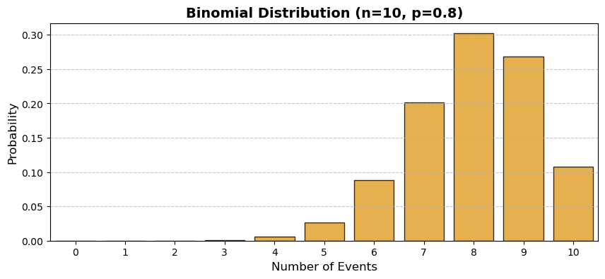
In the limit, as the total number of events goes to infinity, the distribution converges to a normal distribution. This is still unfair--some DERs will participate in very few events, while others will participate in almost all events. What makes a good sampling procedure? DER behavior is nonstationary (changes over time), so we want the sampling procedure to adapt to changes in DER behavior. To be fair to DER owners, we want DERs who have not participated in many recent events to be more likely to be included in the next treatment group. On the other hand, the more we include the DER in the control group, the better the estimate of its baseline behavior (more data gives us better forecasts). A good sampling procedure will aim to have the following:

• Dynamic: The sampling adapts to changing distribution shifts over time.
• Fair: All DERs are selected for the treatment group a similar number of times.
• Accurate: DERs are frequently included in the baseline group, which allows us to gather enough data and create accurate forecasts.

We now discuss a procedure that achieves these desired properties. We maintain a finite history of past events. Limiting the history to the h most recent events is a simple way to make the sampling procedure adapt to changes in DER behavior over time. Each time we run a DER event, we count the number of times a DER has been included in the historical events. Let $n_i$ be the number of times DER $i$ has been included in the treatment group, and let $n$ be the vector containing the counts for all DERs (position $i$ stores $n_i$). Similarly, let $m_i$ be the number of times DER $i$ has been included in the baseline group, and let m be the corresponding vector. To obtain the treatment group, we sample DERs with probabilities according to

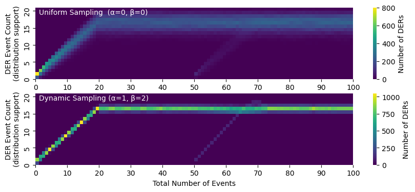
$$ p = \mathrm{softmax}(-\alpha*n + \beta*m). $$

Specifically, $p_i$ is the probability in which DER i is included in the treatment group. Here $\alpha$ is the temperature parameter that controls how much we care about fairness ($\alpha=0$ corresponds to uniform random sampling, which in turn leads to event counts that follow a binomial distribution; larger values of $\alpha$ produce event counts that follow a distribution closer to the delta distribution—all DERs have roughly the same count). Similarly, $\beta$ controls how much we care about obtaining an accurate baseline estimate (larger values give us more baseline data and a better estimate). Because it is more important to obtain ample data for an accurate baseline, we recommend setting $\beta > \alpha$. How much large $\beta$ should be depends on a number of factors, including how easy it is to estimate the baseline, how much we care about fairness, etc.

Next, we address event-induced bias. To do this, we will increase the event count of DERs who participated in an event the previous day; that is, we decrease the probability that they are included in the treatment group. Let $r$ be a vector where $r_i$ equals $0$ if DER $i$ was included in an event the previous day and $\gamma$ otherwise. Intuitively, $\gamma$ should be large to avoid including DERs in subsequent events. In our experiments, setting $\gamma$ equal to the maximum history size works well. The adjusted sampling probabilities are

$$ p = \mathrm{softmax}(-\alpha*(n + r) + \beta*m). $$

Our proposed dynamic sampling procedure generalizes uniform random sampling, which is equivalent to $\alpha = \beta = 0$. Notice that the sampling procedure only depends on the relative DER event count, $n$ and $m$. This has several benefits for scalability.

1. We can introduce new DERs to the group or remove old DERs that have become decommissioned--adding or removing DERS only changes the number of elements of $n$ (its length).
2. The size of the treatment group can change from event to event.

Figure 3: : A comparison between uniform random sampling and our proposed dynamic sampling. This simulation uses a group of 1000 DERs, 100 DER events, a maximum history size of 20, and a treatment group size of 80%. At the 50th event, we introduce 100 new DERs. The uniform sampling procedure eventually converges to a binomial distribution, while the dynamic sampling procedure converges to a distribution with more compact support (values with non-zero probability). This experiment highlights the flexibility in including new devices as well as handling various treatment group sizes (the treatment group increases from 800 to 880 at the 50th event). See the appendix for Python code to replicate the results.

Compensation Strategy

DER baselining relies on the DERs in the baseline group to be operated under NOC. In this section, we discuss a compensation designed to incentivize the aggregator to submit truthful forecasts (baseline estimates) and operate the DERs under NOC.

Our compensation strategy relies on the following:

• We require aggregators to submit forecasts before event announcements.
• The treatment group assignment is randomized according to our procedure.

In particular, we propose the following compensation strategy

compensation = 𝜂*(treatment_impact - 𝜆*baseline_group_error - 𝜇*baseline_der_error)

where treatment_impact is defined in step 4 of static baselining, the baseline_group_error is the absolute value of the bias defined in step 4, and the baseline_der_error is the average mean absolute error of the DER forecasts in the baseline group. Here $\eta$ translates impact into dollars, and $\lambda$ and $\mu$ determine how much we care about penalizing group errors and individual DER errors, respectively. Because the group assignment is randomized, the aggregator cannot artificially manipulate the forecasts (and corresponding baseline group behavior) without incurring a financial penalty

Conclusion

This report introduces a comprehensive framework for DER baselining that addresses key challenges in fairness, accuracy, and manipulation resistance through two core mechanisms:

Dynamic Sampling Framework:

• Continuously cycles DERs between baseline and treatment groups using probability-based selection
• Reduces baseline contamination (event-induced bias) through waiting periods
• Ensures equitable event participation through fairness parameter $\alpha$
• Scales effectively using relative event counts.

Strategic Compensation:

• Incentivizes truthful forecasting through error-based penalties
• Combines treatment impact rewards with baseline accuracy requirements
• Uses randomized group assignment to prevent systematic manipulation
• Balances aggregator compensation against baseline accuracy

This flexible, robust framework supports accurate baseline estimation critical for fair compensation, grid planning, and demand response. Future work could involve determining optimal treatment group sizes and refining compensation parameters for specific market conditions.

Appendix

Python code for the sampling procedure.

def create_treatment_group(
    n, m, r, history, treatment_size,
    alpha=1, beta=2, max_history_size=20
):
    assert len(n) >= treatment_size
    history = history[-max_history_size:] # limit history
    p = softmax(-alpha*(n + r) + 2*beta) # sampling probability
    return np.random.choice(len(n), treatment_size, replace=False, p=p)

Python code to replicate the simulation in Figure 3.

# specify parameters
N_ders = 1000
n_events = 100
treatment_frac = 0.8
alpha = 1
beta = 2
max_history_size = 20


# initialize
history = []
n = np.zeros(N, dtype=np.int32)
m = np.zeros(N, dtype=np.int32)
results = np.zeros((n_events, max_history_size+1))

# run simulation
for it in range(n_events):

    # add 100 more DERs after the 50th event
    if it == 50:
        N_ders += 100
        n = np.append(n, np.zeros(100)).astype(np.int32)
        m = np.append(m, np.zeros(100)).astype(np.int32)
        
    # calculate sampling probability and sample
    r = np.zeros(N_ders)
    if it > 0:
        prev_sample = history[-1]
        r[prev_sample] = max_history_size
        
    treatment_size = int(treatment_frac*N_ders)
    sample = create_treatment_group(
        n, m, r, history, treatment_size, alpha, beta, max_history_size)
        
    # update history, n, and m
    history.append(sample)
    
    n = np.zeros(N_ders)
    der_num, event_count = np.unique(
        np.concatenate(history).flatten(), return_counts=True)
    n[der_num] = event_count
    
    m = len(history) - n
    
    if len(history) >= max_history_size:
        history = history[1:]

    # update results
    num_events, count = np.unique(n, return_counts=True)
    results[it][num_events.astype(np.int32)] = count
    
# plot
sns.heatmap(results.T, cmap="viridis", cbar_kws={'label': 'Number of DERs'})
plt.text(1, 19, "Dynamic Sampling (α=1, β=2)", color="white")
plt.xticks(np.arange(0, n_events+1, 10), np.arange(0, n_events+1, 10))
plt.yticks(np.arange(0, max_history_size+1, 5), np.arange(0, max_history_size+1,
5))

plt.ylabel('DER Event Count\n(distribution support)')
plt.xlabel('Total Number of Events')
plt.gca().invert_yaxis()
plt.show()