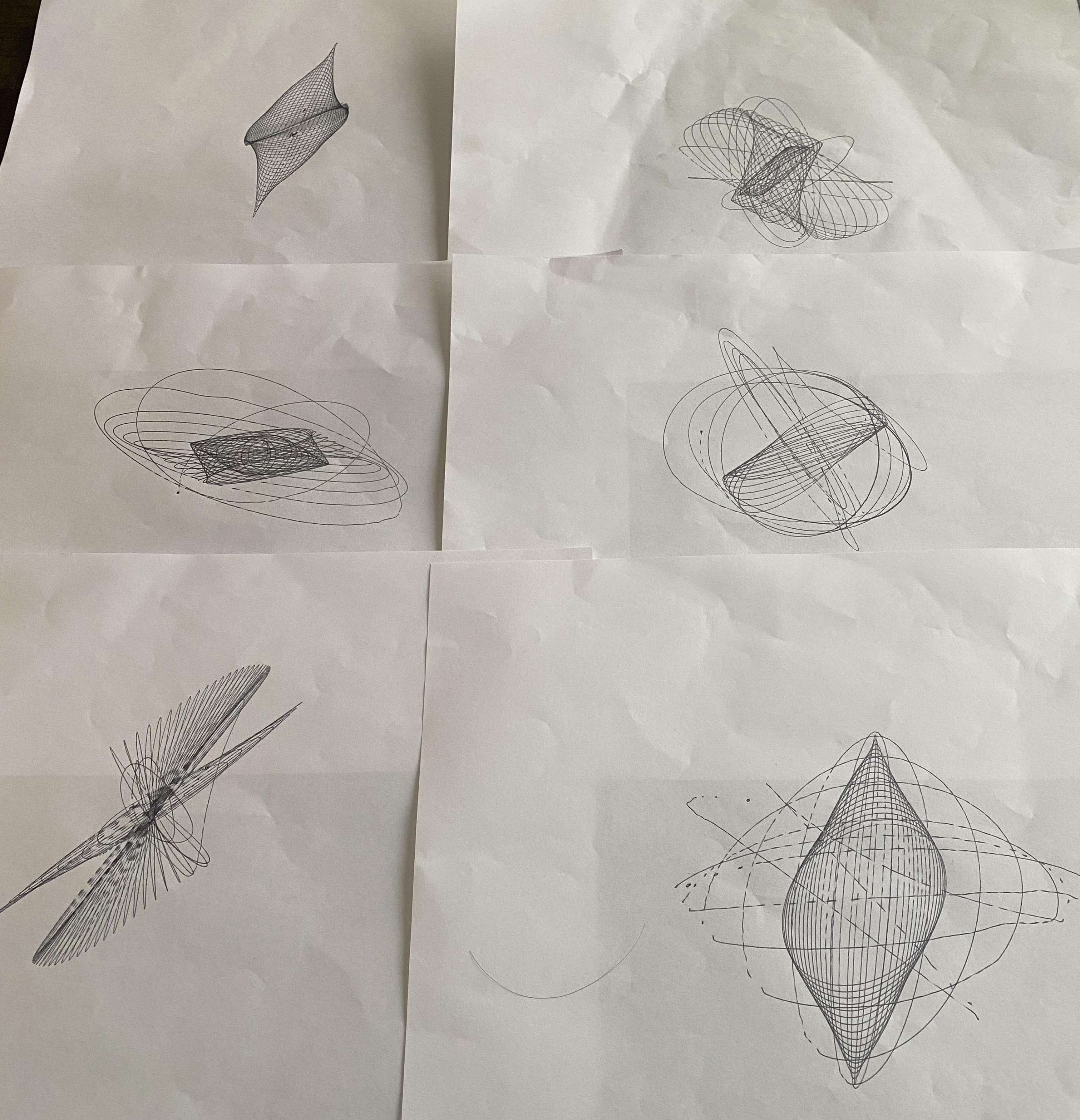
The idea came when nephew showed me some art that he made at the Oregon Museum of Science and Industry. I didn’t know how he made it, but I guessed it was from a pen attached to some sort of pendulum. A simple pendulum would trace elliptical orbits so to create more complex patterns I fudged the physics a bit. Here’s a picture of what he made:

Technical Implementation
The code uses metaprogramming to create abstract line-based artworks using a physics-inspired system. The curves come from a dampled pendulum with distorted equations of motions.
import numpy as np
import matplotlib.pyplot as plt
from scipy.integrate import odeint

def derivatives(state, t):
    u1, v1, u2, v2 = state
    dv1 = -c*np.sin(u1) - 0.01*eta*v1
    dv2 = -c*np.sin(u2) - 0.01*eta*v2
    return [v1, dv1, v2, dv2]

plt.figure(figsize=(8, 3))
for idx, params in enumerate([
    [0, '*', 2, 0, '-', 2, (1, 0, 3, 1), 5, 2],
    [2, '-', 1, 2, '*', 1, (0, 1, 0, 1), 5, 5],
    [1, '+', 2, 0, '-', 2, (0, 1, 3, 5), 2, 1],
]):
    dimx0, opx, dimx1, dimy0, opy, dimy1, init_cond, eta, c = params
    sol = odeint(derivatives, init_cond, np.linspace(0, 100, 10000))
    x = eval(f'np.sin(sol[:,{dimx0}]) {opx} np.cos(sol[:,{dimx1}])')
    y = eval(f'np.sin(sol[:,{dimy0}]) {opy} np.sin(sol[:,{dimy1}])')

    plt.subplot(1, 3, idx+1)
    plt.plot(x, y, 'g', linewidth=1)
    plt.title(str(params).replace(' ', ''), color='g')
    plt.axis('off')
plt.tight_layout()
plt.show()
