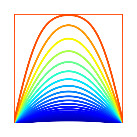
Technical Implementation
This code is based on the heat equation. In my undergrad research, I used the heat equation for geophysics simulations, and during my master’s research, I applied it to modeling water heaters.
The heat equation, a partial differential equation that describes how the distribution of heat evolves over time in a given space. In this case, we’re looking at a 1D rod and so the equation is:
\[\frac{\partial T}{\partial t} = \alpha \frac{\partial^2 T}{\partial x^2}\]where $T$ is the temperature, $t$ is time, $x$ is space, and $\alpha$ is the thermal diffusivity. We use the finite difference method to solve the equation.
import numpy as np
import matplotlib.pyplot as plt
from matplotlib.cm import ScalarMappable
from matplotlib.colors import Normalize

# parameters
L, nx, dx = 10.0, 1000, 0.01
alpha, dt, nt = 0.01, 0.001, 1000000

# simulate
x = np.linspace(0, L, nx)
T = np.zeros(nx)
T[(x > L/4) & (x < L*3/4)] = 1
T_new = T.copy()
times = np.linspace(0, nt-1, 25, dtype=int)
temperatures = []

for n in range(nt):
    update = dt/dx**2*(T[:-2]-2*T[1:-1]+T[2:])
    T_new[1:-1] = T[1:-1] + alpha * update
    T_new[0], T_new[-1] = T_new[1], T_new[-2]
    if n in times:
        temperatures.append(T_new.copy())
    T = T_new.copy()

# plot
cmap = plt.cm.jet
norm = Normalize(vmin=0.49, vmax=1.1)
sm = ScalarMappable(cmap=cmap, norm=norm)

plt.figure()
for T in temperatures[::-1]:
    color = sm.to_rgba(T.max())
    plt.plot(0.1*x, T, color=color)
plt.xlim(0.1*L/4, 0.1*L*3/4)
plt.ylim(0.5, 1.0)
plt.axis('off')
plt.gca().set_aspect('equal')
plt.tight_layout()
plt.show()
